Formatting Cells

Introduction

Spreadsheets that have not been formatted can be difficult to read. Formatted text and cells can draw attention to specific parts of the spreadsheet and make the spreadsheet more visually appealing and easier to understand.
In Excel, there are many tools you can use to format text and cells. In this lesson, you will learn how to change the color and style of text and cells, align text, and apply special formatting to numbers and dates.

Formatting text

Video: Formatting Cells in Excel 2010

Many of the commands you will use to format text can be found in the Font, Alignment, and Number groups on the Ribbon. Font commands let you change the style, size, and color of text. You can also use them to add borders and fill colors to cells. Alignment commands let you format how text is displayed across cells both horizontally and vertically. Number commands let you change how selected cells display numbers and dates.

Optional: You can download this example for extra practice.

To change the font:

1. Select the cells you want to modify.
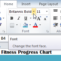
2. Click the drop-down arrow next to the Font command on the Home tab. The font drop-down menu appears.
3. Move your mouse over the various fonts. A live preview of the font will appear in the worksheet.
   
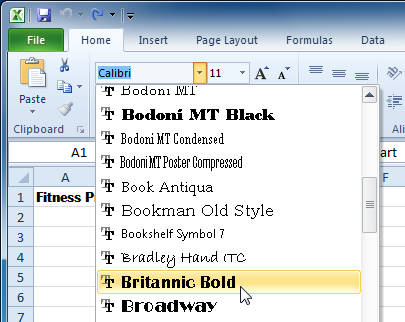
4. Select the font you want to use.

To change the font size:

1. Select the cells you want to modify.
2. Click the drop-down arrow next to the font size command on the Home tab. The font size drop-down menu appears.
3. Move your mouse over the various font sizes. A live preview of the font size will appear in the worksheet.
   
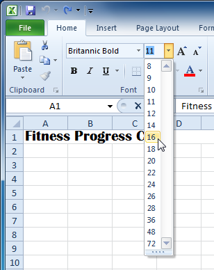
4. Select the font size you want to use.

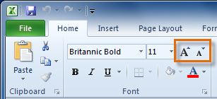
You can also use the Grow Font and Shrink Font commands to change the size.

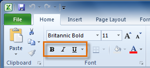
To use the bold, italic, and underline commands:

1. Select the cells you want to modify.
2. Click the Bold, Italic, or Underline command on the Home tab.
   

To add a border:

1. Select the cells you want to modify.
2. Click the drop-down arrow next to the Borders command on the Home tab. The border drop-down menu appears.
   
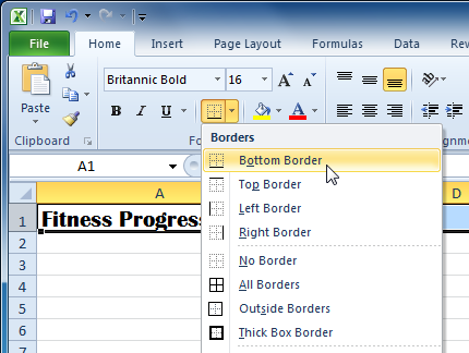
3. Select the border style you want to use.

You can draw borders and change the line style and color of borders with the Draw Borders tools at the bottom of the Borders drop-down menu.

To change font color:

1. Select the cells you want to modify.
2. Click the drop-down arrow next to the font color command on the Home tab. The color menu appears.
3. Move your mouse over the various font colors. A live preview of the color will appear in the worksheet.
   
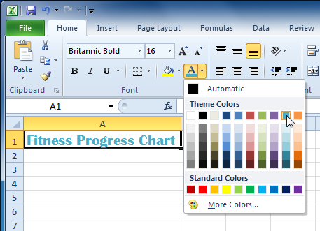
4. Select the font color you want to use.

Your color choices are not limited to the drop-down menu that appears. Select More Colors at the bottom of the menu to access additional color options.

To add a fill color:

1. Select the cells you want to modify.
2. Click the drop-down arrow next to the fill color command on the Home tab. The color menu appears.
3. Move your cursor over the various fill colors. A live preview of the color will appear in the worksheet.
   
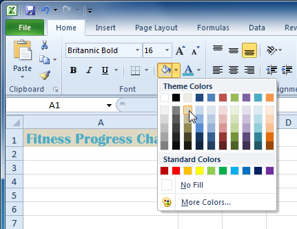
4. Select the fill color you want to use.

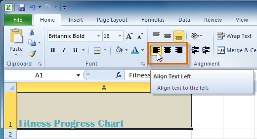
To change horizontal text alignment:

1. Select the cells you want to modify.
2. Select one of the three horizontal Alignment commands on the Home tab.
   • Align Text Left: Aligns text to the left of the cell
   • Center: Aligns text to the center of the cell
   • Align Text Right: Aligns text to the right of the cell
   

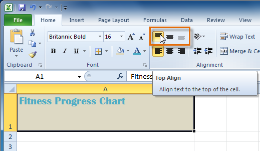
To change vertical text alignment:

1. Select the cells you want to modify.
2. Select one of the three vertical Alignment commands on the Home tab.
   • Top Align: Aligns text to the top of the cell
   • Middle Align: Aligns text to the middle of the cell
   • Bottom Align: Aligns text to the bottom of the cell
   

By default, numbers align to the bottom-right of cells, while words and letters align to the bottom-left of cells.

Formatting numbers and dates

One of Excel's most useful features is its ability to format numbers and dates in a variety of ways. For example, you might need to format numbers with decimal places, currency symbols ($), or percent symbols (%).

To format numbers and dates:

1. Select the cells you want to modify.
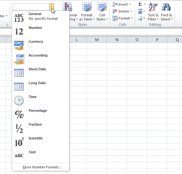
2. Click the drop-down arrow next to the Number Format command on the Home tab.
   
   
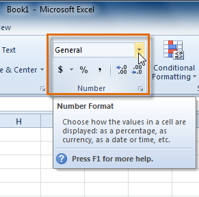
3. Select the number format you want. For some number formats, you can then use the Increase Decimal and Decrease Decimal commands (below the Number Format command) to change the number of decimal places that are displayed.

Click the buttons in the interactive below to learn about the different number formats.

Challenge!

1. Open an existing Excel 2010 document. If you want, you can use this example.
2. Select a cell and change the font, size, or color of the text. If you are using the example, change the title in cell A1 to the Verdana font, size 16, with a font color of green.
3. Select a portion of the content in one cell, and make only that portion bold. For example, if the words Weight (pounds) are in a cell, make only the word Weight bold.
4. Add a border to a group of cells. If you are using the example, add a border to the descriptions in row 3.
5. Change the fill color of a group of cells. If you are using the example, add a fill color to row 3.
6. Try changing the vertical and horizontal text alignment for some cells.
7. Try changing the formatting of a number. If you are using the example, change the date format in column A.