Formatting Tables

Introduction

Once you have entered information into a spreadsheet, you may want to format it. Formatting your spreadsheet can not only improve the look and feel of your spreadsheet, but it also can make it easier to use. In a previous lesson, we discussed many manual formatting options such as bold and italics. In this lesson, you'll learn how to format as a table to take advantage of the tools and predefined table styles available in Excel 2010.

Formatting tables

Video: Formatting Tables in Excel 2010

Just like regular formatting, tables can help to organize your content and make it easier for you locate the information you need. To use tables effectively, you'll need to know how to format information as a table, modify tables, and apply table styles.

Optional: You can download this example for extra practice.

To format information as a table:

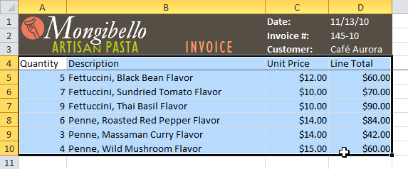
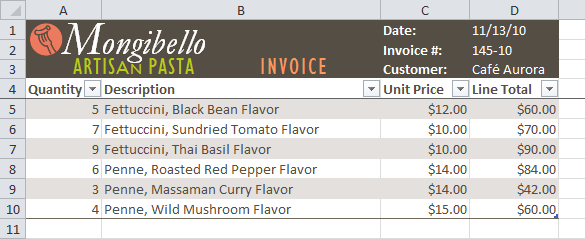
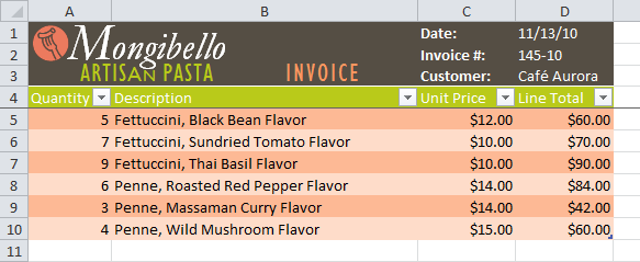
1. Select the cells you want to format as a table. In this example, an invoice, we'll format the cells containing the column headers and order details.
   
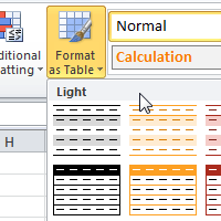
2. Click the Format as Table command in the Styles group on the Home tab.
   
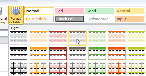
3. A list of predefined table styles will appear. Click a table style to select it.
   
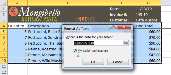
4. A dialog box will appear, confirming the range of cells you have selected for your table. The cells will appear selected in the spreadsheet, and the range will appear in the dialog box.
5. If necessary, change the range by selecting a new range of cells directly on your spreadsheet.
6. If your table has headers, check the box next to My table has headers.
   
7. Click OK. The data will be formatted as a table in the style you chose.
   

Tables include filtering by default. You can filter your data at any time using the drop-down arrows in the header. To learn more, review our Filtering Data lesson.

To convert a table back into normal cells, click the Convert to Range command in the Tools group. The filters and Design tab will then disappear, but the cells will retain their data and formatting.

Modifying tables

To add rows or columns:

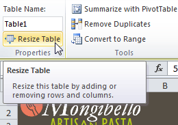
1. Select any cell in your table. The Design tab will appear on the Ribbon.
2. From the Design tab, click the Resize Table command.
   
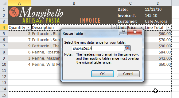
3. Directly on your spreadsheet, select the new range of cells you want your table to cover. You must select your original table cells as well.
   
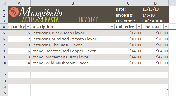
4. Click OK. The new rows and/or columns will be added to your table.
   

To change the table style:

1. Select any cell in your table. The Design tab will appear.
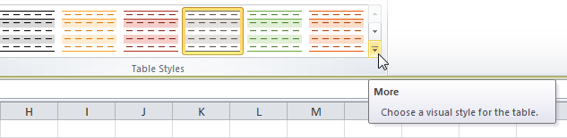
2. Locate the Table Styles group. Click the More drop-down arrow to see all of the table styles.
   
3. Hover the mouse over the various styles to see a live preview.
4. Select the desired style. The table style will appear in your worksheet.
   

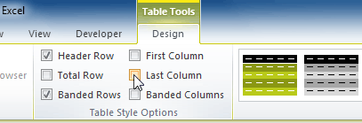
To change table style options:

When using an Excel table, you can turn various options on or off to change its appearance. There are six options: Header Row, Total Row, Banded Rows, First Column, Last Column, and Banded Columns.

1. Select any cell in your table. The Design tab will appear.
2. From the Design tab, check or uncheck the desired options in the Table Style Options group.
   

Depending on the table style you're using, certain table style options may have a different effect. You may need to experiment to get the exact look you want.

Challenge!

1. Open an existing Excel 2010 workbook. If you want, you can use this example.
2. Format a range of cells as a table. If you are using the example, format the column headers (Quantity, Description, etc.) and the order details.
3. Add a row or a column.
4. Change the table style options. If you are using the example, add a total row.
5. Change the table style several times. Take note of how the table options may appear different depending on the style you use.

Read More

Filtering Data

Introduction

Filters can be used to narrow down the data in your worksheet and hide parts of it from view. While it may sound a little like grouping, filtering is different because it allows you to qualify and display only the data that interests you. For example, you could filter a list of survey participants to view only those who are between the ages of 25 and 34. You could also filter an inventory of paint colors to view anything that contains the word blue, such as bluebell or robin's egg blue.

In this lesson, you'll learn how to filter the data in your worksheet to display only the information you need.

Filtering data

Video: Filtering Data in Excel 2010

Filters can be applied in different ways to improve the performance of your worksheet. You can filter text, dates, and numbers. You can even use more than one filter to further narrow your results.

Optional: You can download this example for extra practice.

To filter data:

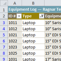
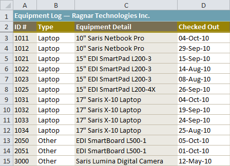
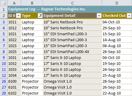
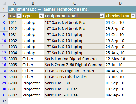
In this example, we'll filter the contents of an equipment log at a technology company. We'll display only the laptops and projectors that are available for checkout.

1. Begin with a worksheet that identifies each column using a header row.
   
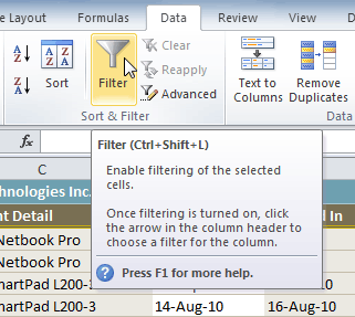
2. Select the Data tab, then locate the Sort & Filter group.
3. Click the Filter command.
   
4. Drop-down arrows will appear in the header of each column.
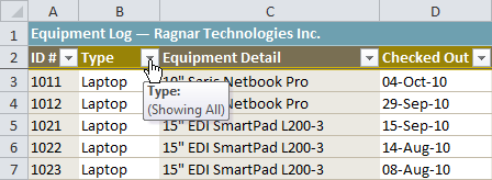
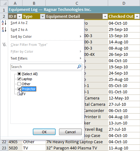
5. Click the drop-down arrow for the column you want to filter. In this example, we'll filter the Type column to view only certain types of equipment.
   
6. The Filter menu appears.
7. Uncheck the boxes next to the data you don't want to view, or uncheck the box next to Select All to quickly uncheck all.
8. Check the boxes next to the data you do want to view. In this example, we'll check Laptop and Projector to view only these types of equipment.
   
9. Click OK. All other data will be filtered, or temporarily hidden. Only laptops and projectors will be visible.
   

Filtering options can also be found on the Home tab, condensed into the Sort & Filter command.

To add another filter:

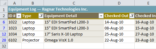
Filters are additive, meaning you can use as many as you need to narrow your results. In this example, we'll work with a spreadsheet that has already been filtered to display only laptops and projectors. Now we'll display only laptops and projectors that were checked out during the month of August.

1. Click the drop-down arrow where you want to add a filter. In this example, we'll add a filter to the Checked Out column to view information by date.
2. Uncheck the boxes next to the data you don't want to view. Check the boxes next to the data you do want to view. In this example, we'll check the box next to August.
   
3. Click OK. In addition to the original filter, the new filter will be applied. The worksheet will be narrowed down even further.
   

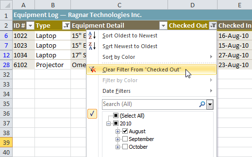
To clear a filter:

1. Click the drop-down arrow in the column from which you want to clear the filter.
2. Choose Clear Filter From.
   
3. The filter will be cleared from the column. The data that was previously hidden will be on display once again.

To instantly clear all filters from your worksheet, click the Filter command on the Data tab.

Advanced filtering

To filter using search:

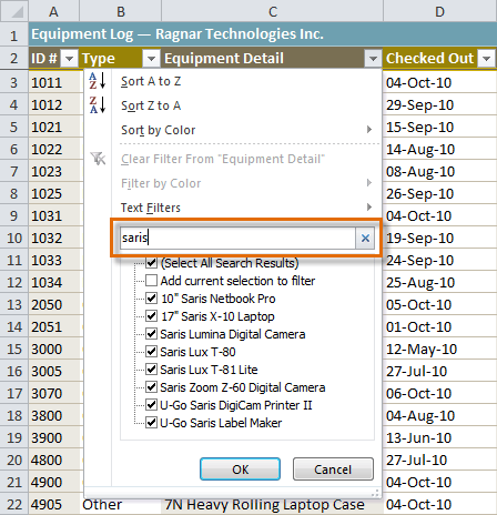
Searching for data is a convenient alternative to checking or unchecking data from the list. You can search for data that contains an exact phrase, number, date, or simple fragment. For example, searching for the exact phrase Saris X-10 Laptop will display only Saris X-10 laptops. Searching for the word Saris, however, will display Saris X-10 laptops and any other Saris equipment, including projectors and digital cameras.

1. From the Data tab, click the Filter command.
2. Click the drop-down arrow in the column you want to filter. In this example, we'll filter the Equipment Detail column to view only a specific brand.
3. Enter the data you want to view in the Search box. We'll enter the word Saris to find all Saris brand equipment. The search results will appear automatically.
   
4. Check the boxes next to the data you want to display. We'll display all of the data that includes the brand name Saris.
5. Click OK. The worksheet will be filtered according to your search term.
   

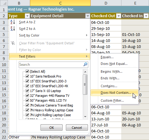
Using advanced text filters

Advanced text filters can be used to display more specific information, such as cells that contain a certain number of characters or data that does not contain a word you specify. In this example, we'll use advanced text filters to hide any equipment that is related to cameras, including digital cameras and camcorders.

1. From the Data tab, click the Filter command.
2. Click the drop-down arrow in the column of text you want to filter. In this example, we'll filter the Equipment Detail column to view only certain types of equipment.
3. Choose Text Filters to open the advanced filtering menu.
4. Choose a filter. In this example, we will choose Does Not Contain to view data that does not contain the text we specify.
   
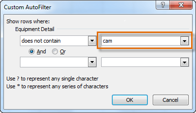
5. The Custom AutoFilter dialog box appears.
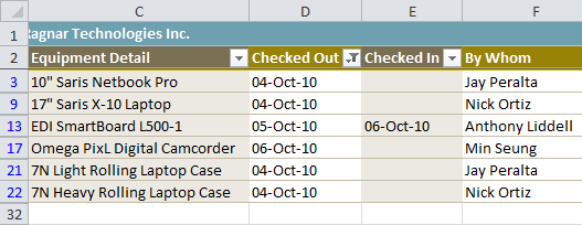
6. Enter your text to the right of your filter. In this example, we'll enter cam to view data that does not contain these letters. That will exclude any equipment related to cameras, such as digital cameras, camcorders, camera bags, and the digicam printer.
   
7. Click OK. The data will be filtered according to the filter you chose and the text you specified.

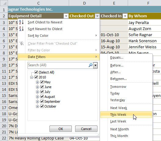
Using advanced date filters

Advanced date filters can be used to view information from a certain time period, such as last year, next quarter, or between two dates. Excel automatically knows your current date and time, making this tool easy to use. In this example, we'll use advanced date filters to view only the equipment that has been checked out this week.

1. From the Data tab, click the Filter command.
2. Click the drop-down arrow in the column of dates you want to filter. In this example, we'll filter the Checked Out column to view only a certain range of dates.
3. Choose Date Filters to open the advanced filtering menu.
4. Click a filter. We'll choose This Week to view equipment that has been checked out this week.
   
5. The worksheet will be filtered according to the date filter you chose.
   

If you're working along with the example file, your results will be different from the images above. If you want, you can change some of the dates so the filter will give more results.

Using advanced number filters

Advanced number filters allow you to manipulate numbered data in different ways. For example, in a worksheet of exam grades you could display the top and bottom numbers to view the highest and lowest scores. In this example, we'll display only certain types of equipment based on the range of ID #s that have been assigned to them.

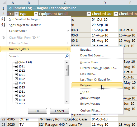
1. From the Data tab, click the Filter command.
2. Click the drop-down arrow in the column of numbers you want to filter. In this example, we'll filter the ID # column to view only a certain range of ID #s.
3. Choose Number Filters to open the advanced filtering menu.
4. Choose a filter. In this example, we'll choose Between to view ID #s between the numbers we specify.
   
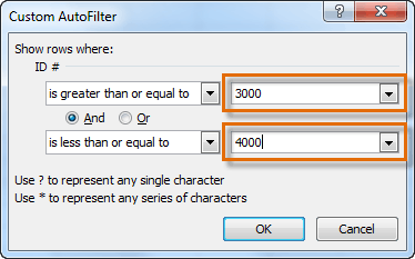
5. Enter a number to the right of each filter. In this example, we'll view ID #s greater than or equal to 3000 but less than or equal to 4000. This will display ID #s in the 3000-4000 range.
   
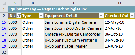
6. Click OK. The data will be filtered according to the filter you chose and the numbers you specified.
   

Challenge!

1. Open an existing Excel 2010 workbook. If you want, you can use this example.
2. Filter a column of data. If you are using the example, filter the Type column so it displays only laptops and other equipment.
3. Add another filter by searching for the data you want. If you are using the example, search for EDI brand equipment in the Item Description column.
4. Clear both filters.
5. Use an advanced text filter to view data that does not contain a certain word or phrase. If you are using the example, display data that does not contain the word cam. This should exclude any camera-related equipment, such as digital cameras and camcorders.
6. Use an advanced date filter to view data from a certain time period. If you are using the example, display only the equipment that was checked out in September 2010.
7. Use an advanced number filter to view numbers less than a certain amount. If you are using the example, display all ID #s less than 3000.

Read More

Outlining Data

Introduction

If the amount of data in your worksheet becomes overwhelming, creating an outline can help. Not only does this allow you to organize your data into groups and then show or hide them from view, but it also allows you to summarize data for quick analysis using the Subtotal command (for example, subtotaling the cost of office supplies depending on the type of product).

In this lesson, you will learn how to outline your worksheet in order to summarize and control how your data is displayed.

Outlining data

Video: Outlining Data in Excel 2010

Outlines give you the ability to group data you may want to show or hide from view, as well as to create a quick summary using the Subtotal command. Because outlines rely on grouping data that is related, you must sort before you can outline. For more information, you may want to review our lesson on Sorting Data.

Optional: You can download this example for extra practice.

Outlining data using Subtotal

The Subtotal command can be used to outline your worksheet in several ways. It uses common functions like SUM, COUNT, and AVERAGE to summarize your data and place it in a group. To learn more about functions, visit our Working with Basic Functions lesson.
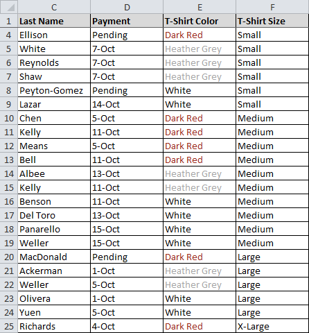
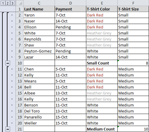
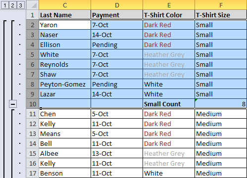
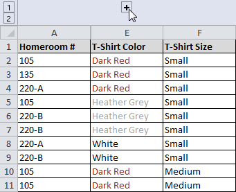
In this example, we'll use the Subtotal command to count the number of T-shirt sizes that were ordered at a local high school. This will also place each T-shirt size in a group, making it possible to show the count but hide the details that are not crucial to placing the order (such as a student's homeroom number and payment date).

To outline data using Subtotal:

1. Sort according to the data you want to outline. Outlines rely on grouping data that is related. In this example, we will outline the worksheet by T-Shirt Size, which has been sorted from smallest to largest.
   
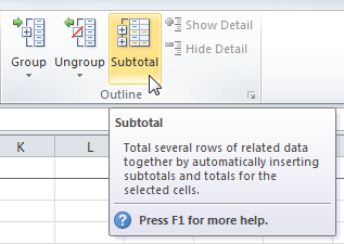
2. Select the Data tab, then locate the Outline group.
3. Click the Subtotal command to open the Subtotal dialog box.
   
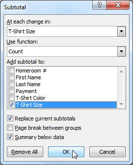
4. In the At each change in field, select the column you want to use to outline your worksheet. In this example, we'll choose T-Shirt Size.
5. In the Use function field, choose from the list of functions that are available for subtotaling. We'll use the COUNT function to tally the number of each size.
6. Select the column you want the subtotal to appear in. We'll choose the T-Shirt Size column.
7. Click OK.
   
8. The contents of your worksheet will be outlined. Each T-shirt size will be placed in its own group, and the subtotal (count, in this case) will be listed below each group.
   

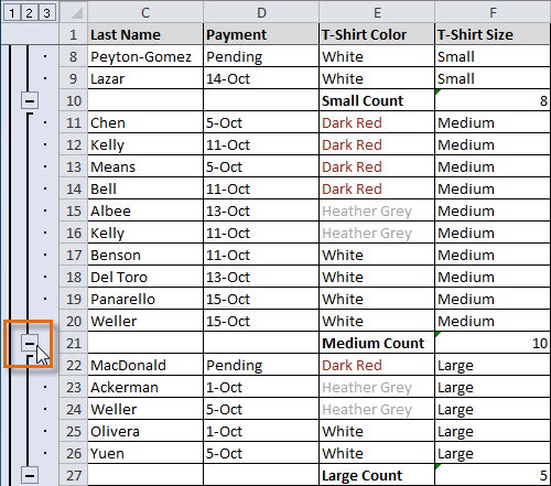
Showing and hiding data

To show or hide a group:

1. Click the minus sign—also known as the Hide Detail symbol—to collapse the group.
   
2. Click the plus sign—also known as the Show Detail symbol—to expand the group again.
   

You can also use the or commands on the Data tab in the Outline group. Select a cell in the group you want to show or hide, then click the appropriate command.

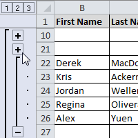
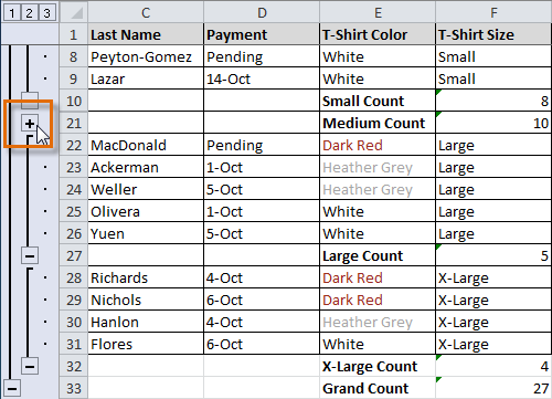
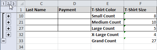
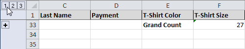
To view groups by level:

The groups in your outline, based on their hierarchy, are placed on different levels. You can quickly display as little or as much information as you want by clicking the level symbols to the left of your worksheet. In this example, we will view levels in descending order, starting with the entire worksheet on display, then finishing with the grand total. While this example contains only three levels, Excel can accommodate up to eight.

1. Click the highest level (level 3 in this example) to view and expand all of your groups. Viewing groups at the highest level will display the entirety of your worksheet.
   
2. Click the next level (level 2 in this example) to hide the detail of the previous level. In this example, level 2 contains each subtotal.
   
3. Click the lowest level (level 1 in this example) to display the lowest level of detail. In this example, level 1 contains only the grand total.
   

Removing groups and subtotaling

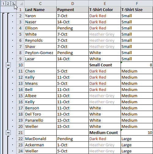
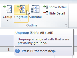
To ungroup data:

1. Select the rows or columns you want to ungroup. In this example, we'll ungroup size Small.
   
2. From the Data tab, click the Ungroup command. The range of cells will be ungrouped.
   

To ungroup all of the groups in your outline, open the drop-down menu under the Ungroup command, then choose Clear Outline.

Ungroup and Clear Outline will not remove subtotaling from your worksheet. Summary or subtotal data will stay in place and continue to function until you remove it.

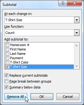
To ungroup data and remove subtotaling:

1. From the Data tab, click the Subtotal command to open the Subtotal dialog box.
2. Click Remove All.
   
3. All data will be ungrouped, and subtotals will be removed.
   

Creating your own groups

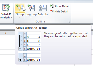
The Group command allows you to group any range of cells—either columns or rows. It does not calculate a subtotal or rely on your data being sorted. This gives you the ability to show or hide any part of your worksheet and display only the information you need.

To create and control your own group:

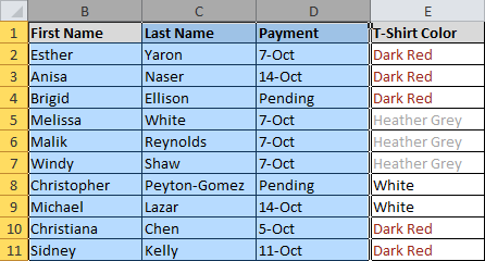
In this example, we will prepare a list of T-shirt colors and sizes that need to be distributed to each homeroom. Some of the data in the worksheet is not relevant to the distribution of T-shirts; however, instead of deleting it, we'll group it, then temporarily hide it from view.

1. Select the range of cells you want to group. In this example, we will group the First Name, Last Name, and Payment columns.
   
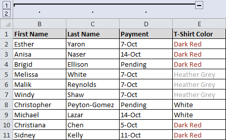
2. From the Data tab, click the Group command.
   
3. Excel will group the selected columns or rows.
   
4. Click the minus sign—also known as the Hide Detail symbol—to hide the group.
5. The group will be hidden from view.
   

Click the plus sign—also known as the Show Detail symbol—to show the group again.

Challenge!

1. Open an existing Excel 2010 workbook. If you want, you can use this example.
2. Outline your worksheet using the Subtotal command. If you are using the example, outline by T-shirt size.
3. Display the first level of groups in your outline.
4. Display the highest level to view your entire worksheet again.
5. Create your own group of rows or columns, then hide the group from view.
6. Ungroup any range of data.
7. Remove subtotaling from your worksheet.

Read More